Mineral Resources

|
Mineral Resources |
|
|
|
|
|
|
|
|
|
|
||||||||
|
|
|
|
Updated on 05-05-15 |
||||||||||
|
Contents of the |
Other topics in this Module:
|
On this page ...
|
||||||||||||||||||||||||
|
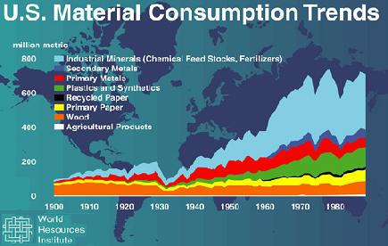
Earth
resources range from the extractive ones like mineral and most of the energy
resources that are largely nonrenewable or exhaustible
to potentially renewable
resources like air, water and soil and the supposedly perennial
or renewable resources like solar, wind, water, waves, tides,
oceans (i.e., the solar heat trapped in warm surface waters of the tropics).
|
Two of the typically
extractable ones of these, discussed here, are broadly grouped as:
|
|
||||||||||||||||
|
|
|||||||||||||||||
|
Of these, the "McKelvey Box" approach is schematically explained in the figure on the left and concerns the definition of reserves and what distinguishes reserves from resources. Reserves are what we have discovered already and can economically extract whereas resources encompass a much broader spectrum. We have certainly had a great deal more of oil in Shakespeare's time than what now remains, for instance, but "oil" was not a resource in his time.
If this constraint is part technological and part economic, the second constraint is even more directly economic and is explained in illustration below. |
 |
|
|
Suppose at a given point in
time, the demand for a resource is defined by D1 and its supply by S1. The
demand schedule here slopes downwards, of course, suggesting that the lower
the price the greater will be the quantity consumed. Likewise, the supply
schedule slopes upwards here, reflecting the fact that the steeper the price
the greater will be the incentive to produce and that increases the supply.
Price (P1) and quantity (Q1) are then defined by the point at which these
two schedules intersect. What if the demand suddenly shoots up, say to the
new demand schedule D2? If the supply schedule concomitantly rises to S2
then the new equilibrium price will be P2 and quantity Q2. |
|
On the other hand, if the supply schedule stays the same ― the likely scenario for exhaustible resources, then the new equilibrium price will be P3 at the quantity Q3. Note that Q3 is less than Q2 but P3 is greater than P2. What if there is a glut in the market, with demand D2 reverting back to D1? The price will now fall to P4 if supply S2 does not change but may revert to P1 if S2 reverts to S1. As we shall see later on this page as also elsewhere, inflation-adjusted long-run prices of the earth resources have hardly increased as rapidly as their demand. |
|
|
|
Click on the right for
|
 or click on the left for the USGS mineral resources pages |
|
Types
of mineral resources:
|
and ranges from about 60 ppm (parts per million) for copper, 2 ppm for tin, 4 ppb (parts per billion) for gold etc., i.e., the more scarce a resource is the smaller its concentration needs to be for its cost-effective extraction. |
|
 |
||
|
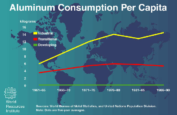
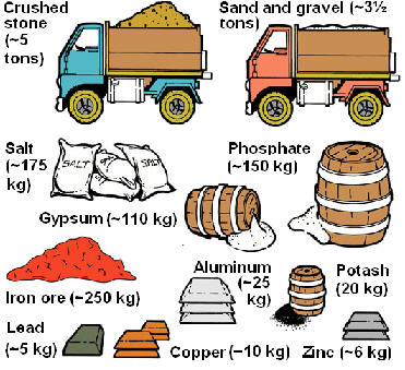
The average per capita consumption of selected |
|||
|
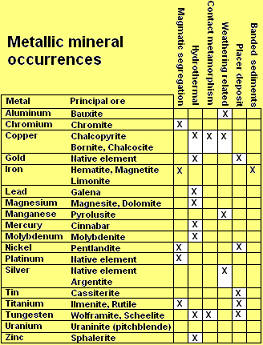
Occurrences of
mineral
|
|
 |
||
 |
|||
| Polymetallic deposits of copper, lead, zinc, gold, silver, nickel, cobalt, tin, tungsten, molybdenum, mercury and iron occur as hydrothermal deposits (contact metamorphism, hydrothermal veins, disseminated deposits and hot-spring deposits). |
 |
||
 |
|||
| Pegmatites often carry lithium, mica, rare metals and barites. | |||
|
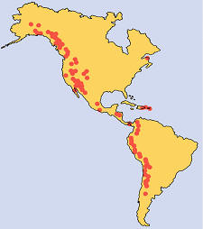
Polymetallic deposits often occur in the folded mountain belts. Notice how porphyry copper and molybdenum deposits dot the entire subduction zone from Andes to the Cascades. Almost all the U.S. reserves of gold, silver, platinum and palladium come from the western U.S., from Rockies to the Sierras and Cascades. |
|||
|
|
Issues of
exhaustibility and environmental degradation:
|
On the other hand, no such
threat of imminent exhaustibility exists if we take the cornucopian view,
that technological innovation will always provide substitutes and
alternatives. The question is if such has indeed been the case. |
|
|
|
|
|
|
|
 |